The vast majority of SEMs (Scanning Electron Microscopes) come equipped (or may be equipped) with EDS (Energy Dispersive x-ray Spectroscopy, also known as EDX) which allows quantitative analysis of chemical elements present in the sample. Exciting recent developments in MountainsSpectral® software now open up possibilities for combining and comparing these characteristics with surface topography in order to better understand material behavior. Renata Lewandowska, product manager for spectral applications at Digital Surf, explains the new tools and their applications.

3D reconstruction
Several years ago, the Digital Surf team unveiled a new, revolutionary method for quickly building a 3D model from 2 successive scans or four 4-quadrant images from an SEM.
See the full method in our webinar: bit.ly/3D-reconstruction
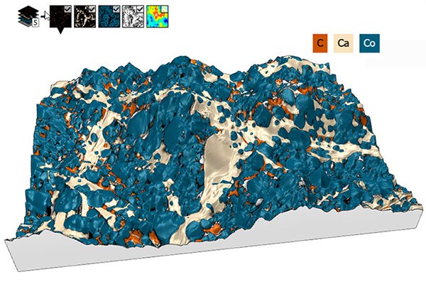
Above: 3D model of surface topography with overlay of chemical composition on a Cobaltite sample.
Courtesy of Emmanuel Guilmeau, CRISMAT (Caen, France), Jean-Claude Ménard, JEOL France.
Colocalization tools for overlaying spectral data
Very often, users of SEM can also generate EDS maps of the sample they are studying. However, bringing together these datasets of different nature and at different scales to study them collectively can be particularly tricky. MountainsSpectral® now offers a streamlined method for performing this task, all within a single software package.
Connecting background data with overlays
The first step in the process is to select the desired background and create a Colocalization study. This could simply be a 2D image but in the case presented here (a Cobaltite sample imaged with SEM and EDS), a 3D topography was used. In the next step, users can choose to add overlay images. In the present case, three EDS chemical maps were chosen as overlay images.
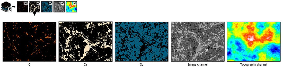
Above: Grid view of all data (background and overlays) used to perform colocalization.
Transparency settings can be manipulated to check positioning of the overlays on the background (particularly useful when the two datasets are not at the same scale).
Several methods are available to position overlays more accurately. In this example, we used the Use points method to identify similar structures on the two datasets and create pairs of points to be colocalized with each other.
Finally, we used the Composite rendering tool in MountainsSpectral® to choose which EDS maps to work with and mix colors from these.
Showcasing data in 3D
Visualizing and manipulating data in 3D can really help us better interpret data analyzed. Luckily, a variety of methods are available for generating a 3D view in MountainsSpectral®.
The Generate 3D view tool in the Colocalization study is one way to display your data in 3D with close to zero effort. This technique uses the topographic values from the reconstructed SEM image and pastes the color image from the colocalization on top.
As an alternative, using the Generate whole content feature, it is possible to obtain all colocalization datasets (background and overlay images) as a Multi-channel image. This has the extra advantage of opening up other possibilities for processing this data (access to Operators and Studies on Multi-channel images). This method also gives more flexibility for adjusting composition once the colocalization is performed.
Whichever method you end up using, once the 3D view has been generated, you benefit from a multitude of enhancement options: amplify height representations, modify rendering and gloss and define the ideal lighting conditions for your sample.
Finally, the Animated view allows you to simulate flight over the data, following one of several predefined paths. All these are excellent tools for creating an outstanding presentation.
Correlation made easy
Beyond creating an esthetically pleasing image, the workflow described in this article allows us to make correlations between different kinds of instrument data (SEM & EDS images).
The ability to easily hide and unhide the various chemical maps (calcium, carbon etc.) on 3D data allows us to show and understand relationships between the different components.
See correlation in action
There’s nothing like a demonstration to better get your head round new tools and how they work! Join us on September 8, 2022, when Renata will be showing correlation step-by-step in our webinar on “Spectroscopy data preparation, analysis and correlation with MountainsSpectral®”. Click here to learn more and register.