Optical profilers are very popular nowadays and frequently used to verify surface texture specifications on manufactured components. However, technical drawings are usually not made for such areal instruments and instead provide profile surface texture specifications. This can be confusing and may lead users to wonder how to compare profile and areal values.
The short answer is that they cannot be compared but in reality things are a little more complicated than that. The thing is that areal values only differ from profile values by a small margin. This could mean some users are comparing Sa values directly with Ra specifications, which is a mistake. The case of Ra/Sa is discussed here but the same reasoning can also applied to other parameters (Rk/Sk, Rq/Sq etc.)
Even though the equation of Sa is the areal extrapolation of the equation of Ra (see below), this does not mean that values should not be compared directly.
When a technical drawing contains a surface texture specification using Ra and a given tolerance limit, it is not possible to directly compare Sa values with the tolerance value given for Ra. A new tolerance value needs to be fixed for areal measurements and new specifications, adapted to Sa, need to be defined.
The first reason for this relates to the analysis bandwidth. Ra, by definition, is calculated on a roughness profile, based on a profile filter which filters spatial frequencies along the X axis (by default a Gaussian filter with a cut-off of 0.8 mm). Moreover, it is evaluated on several sampling lengths (as per ISO 4288) and averaged (except when calculating Ra according to ASME B46.1 where only one value is calculated over the sampling length).
On the other hand, Sa is calculated on a S-L or S-F surface based on a 3D filter. The areal filter takes into account wavelengths in all directions which means that it generates a different effect from the profile filter. The difference is especially visible when the surface has directional structures such as scratches or directional tool marks or possesses periodical patterns.
The second reason we need distinct specifications for Sa is to do with the size and resolution of the measured surface. When measuring a profile on a component, ISO 3274 defines the relationship between stylus tip, data spacing and evaluation length. A typical measurement is 5.6 mm long with a lateral resolution of 0.5 µm, which means 11,200 points.
An areal measurement made with an optical profiler is usually smaller in lateral size (commonly between 1 and 2 mm). Its lateral resolution may be of the same order (1 µm) depending on the instrument lens. Larger areas may be obtained using small magnification objectives (although these are less well adapted to surface texture) or by stitching many surfaces together. A lateral scanning instrument, such as a 3D stylus profilometer or a chromatic confocal probe, makes it possible to scan a larger area and generate a surface several millimeters in size, but users frequently select larger spacing in Y (between lines) than spacing in X (between points) in order to reduce the scanning time. These differences in lateral resolution and scan size lead to differences in parameter values.
The following examples show how results are different, yet close enough to create confusion. The comparison with profiles is obtained by extracting series of profiles along X or Y. A real profile measurement would usually be of a longer size and have better lateral resolution.
Example 1:
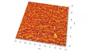 Shot blasted aluminum, measured with a confocal microscope.
The surface is almost isotropic.
Sa = 3.283 µm
Ra(x) = 2.741 µm +/- 0.271 µm
Ra(y) = 2.974 µm +/- 0.243 µm
Gaussian filter with a cut-off of 0.25 mm.
Example 2:
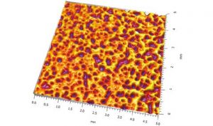 Grained plastic measured with a stylus profilometer.
The surface has homogeneous texture cells.
Sa = 7.016 µm
Ra(x) = 5.422 µm +/- 0.928 µm
Ra(y) = 5.307 µm +/- 1.025 µm
Gaussian filter with a cut-off of 0.8 mm.
Example 3:
![]() Structures on an ultrasound transducer, measured with a chromatic confocal probe.
Structures on an ultrasound transducer, measured with a chromatic confocal probe.
Sa = 1.247 µm
Ra(x) = 0.973 µm +/- 0.187 µm
Ra(y) = 0.876 µm +/- 0.331 µm
Gaussian filter with a cut-off of 0.25 mm
Key takeaways
- Areal parameters cannot be directly compared with specifications and tolerances of profile parameters.
- Distinct specifications need to be set for areal measurements and indicated as such on drawings.
- Recommended instrument technique may be indicated in order to avoid variations between specification and verification.
Author : François Blateyron
Resources :
Digital Surf Metrology Guide: www.https://www.digitalsurf.com/guide
ISO 3274:1996 – GPS – Surface texture: Profile method – Nominal characteristics of contact (stylus) instruments
ISO 25178-1:2016 – GPS – Surface texture: Areal – Indication of surface texture
ISO 16610-1:2015 – GPS – Filtration: Overview and basic concepts
Optical measurement of surface topography, R. Leach ed., Springer